Determination of Equilibrium for National Income in a Two Sector Economy:

J.M. Keynes in his famous book, 'General theory', has used two methods for the determination of national income at a particular time:

(1) Saving Investment Method.

(2) Aggregate Demand and Aggregate Supply Method.

Both these approaches lead us to the determination of the same level of national income.

It may here be mentioned that Keynes model of income determination is relevant in the context of short run only.

Assumptions:

Keynes assumes that in the short run:

(i) The stock of capital, technique of production, forms of business organizations, do not change.

(ii) He also assumes a fair degree of competition in the market.

(iii) There is also absence of government role either as a taxer or as a spender.

(iv) Keynes further assumes that the economy under analysis is a closed one. There is no influence of exports and imports on the economy.

This approach is based on the Keynesian definitions of saving and investment. According to Keynes, the level of national income, in the short run, is determined at a point where planned or intended saving is equal to planned or intended investment. Saving as defined by Keynes is that part of income which is not spent on consumption (S = Y - C). On the other hand, investment is the expenditure on goods and services not meant for consumption. (I = Y - C).

According to Keynes, if at any time, the intended saving is less than intended investment, it implies that people are spending more on consumption. The rise in consumption will reduce the stock of goods in the market. This will give incentive to entrepreneurs to increase output. Likewise, if at anytime intended saving is greater than intended investment, this would mean that people are spending lesser volume of money on consumption. As a result of this, the inventories of goods will pile up. This will induce entrepreneurs to reduce output. The result of this will be that national income would decrease. The national income will be in equilibrium only when intended saving is equal to intended investment.

Example and Diagram/Curve:

The determination of national income is now explained with the help of saving and investment curve below:

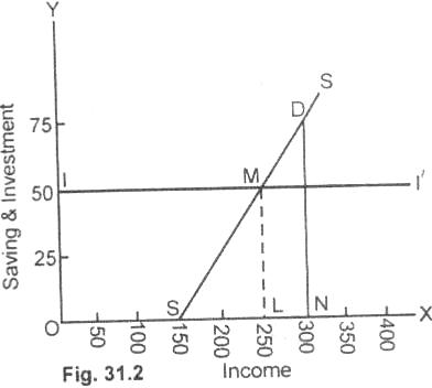
In figure (31.2), income is measured on OX axis and saving and investment on OY axis. SS is the saving curve which shows intended saying at different levels of income. The investment curve ll^/ is drawn parallel to the X axis which shows that investment does not change.

The entrepreneurs intend to invest $50 crore only irrespective of the amount of income. Saving (SS) and investment curves (ll^/) intersect each other at point M. If the conditions stated above remain the same, the size of equilibrium level of income is 250 crore.

Disequilibrium:

Under the assumed conditions if there is inequality between saving and investment or disequilibrium, the forces will operate in the economy and restore the equilibrium position.

Let us suppose, that the income has increased from the equilibrium level OL to ON ($300 crore). At this level of income, desired saving is greater than the desired investment. When intended saving exceeds planned or intended investment, the businessmen will not be able to dispose off all their current output. They will slow down their productive activities. This will result in reducing the number of workers employed in factories and a decrease in the income. This process will go on until due to a decrease in income, people's saving is reduced to the level of investment ($50 crore). The equilibrium income is $250 crore.

In the same way, income cannot remain below this equilibrium level of $250 crore. If at any time, income falls below the equilibrium level, then it means that people are investing more than they are willing to save I > S. They will increase productive activities as they are making high profits. The number of workers employed in the factories will increase. This will result in an increase in income and higher saving. This rise in national income will go on up to a point where saving and investment are just in balance and that will be the equilibrium level. At this point, income will have the tendency of neither to rise nor to fall. It will be in a state of rest. It is, thus, clear that national income is determined at a point where the intended investment is equal to intended saving.

While determining the level of national income in a two sector economy, it is assumed that it is an economy where there is no role of the government and of foreign trade. In other words, it is a closed economy with no government intervention. The two sector economy comprises of households and firms.

According to J. M. Keynes, the equilibrium level of national income is that situation in which aggregate demand (C+ I) is equal to aggregate supply (C + S). The aggregate demand (C+ I) refers to the total spending in the economy. In a two sector economy, The aggregate demand is the sum of demands for the consumer goods (c) and investment goods by households and firms respectively. The aggregate demand curve is positively sloped. It indicates that as the level of national income rises, the aggregate demand (or aggregate spending) in the economy also rises.

Aggregate supply (C + S):

It is the flow of goods and services in the economy. In other words, the value of aggregate supply is equal to the value of net national product (national income). The aggregate supply curve (C + S) is a positively sloped 45° helping line. It signifies that as the level of national income rises, the aggregate supply also rises by the same proportion.

According to Keynesian model, the equilibrium level of national income is determined at a point where the aggregate demand curve intersects the aggregate supply curve. The 45° helping line represents aggregate supply. By definition, output equals income on each point of aggregate supply curve. The determination of the level of aggregate income is explained below.

Diagram/Curve:

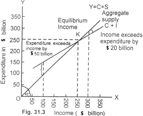
In the figure 31.3, income is measured along OX axis and expenditure on OY axis. The aggregate demand curve (C + I) intersects the aggregate supply curve (45° line) at point K point. K, here is the only point where the economy is willing to spend exactly the amount which is necessary to dispose off the entire output. The equilibrium level of income is $250 billion. It may, however, be noted that this equilibrium output does not mean in any way the full employment output.

Departure From Equilibrium Level of Income:

Now a question arises that if at any time there is a departure from the equilibrium income of $250 billion, how will the economy move towards an equilibrium level? To answer this question, we examine two possible levels of income other than the equilibrium level.

Let us suppose first that the actual income is $300 billion rather than $250 billion. According to aggregate demand, schedule (C + l), (the actual consumption + investment expenditure) at an income of $300 billion falls short by $30 billion (shown by bracket). This means that the goods worth $30 billion are not sold. When the inventories pile up with the business, they would curtail this production and provide fewer jobs. There will thus be a decline in total income which will continue till the income falls to the equilibrium level of $250 billion.

Now let us suppose that the level of income fails to $100 billion. According to aggregate demand schedule represented by (C + l) curve, the expenditure at this level exceeds income by $50 billion (shown by bracket). The increase in demand of consumer and investment goods will induce the businesses to increase their output. The higher rate of production will provide more jobs to the workers.

The level of income would rise and the upward drive continues till the income reaches the equilibrium level of $250 billion. We, thus, conclude by saying that an economy sustains only that level of income where the total quantity supplied and the aggregate quantity demanded are equal. At this equilibrium national income of $250 billion, the firms have neither the tendency to increase output nor the tendency to decrease output. Hence, $250 billion is the equilibrium level of national income. The equilibrium output, in this simple Keynesian analysis, does not mean full employment.