Three Important
Economic Models of
Oligopoly
are as:
(1) Price and output
determination under collusive oligopoly.
(2) Price and output
determination under non-collusive oligopoly.
(3) Price leadership
model.
(1)
Price and Output Determination Under Collusive Oligopoly:
The term
'collusion' implies to 'play together'. When firms under
oligopoly agree formally not to compete with each other about
price or output, it is called collusive oligopoly.
The firms may agree on setting output quota, or fix prices or
limit product promotion or agree not to 'poach' in each other's
market. The completing firms thus from a 'cartel'. The members
of firms behave as if they are a single firm.
Assumptions of Price and Output Determination Under Collusive
Oligopoly:
For price output
determination in a collusive oligopoly, we assume that (i) there
are only three firms in the industry and they form a cartel,
(ii) the products of all the three firms are homogenous (iii)
the cost curves of these firms are identical.
Under the assumptions
stated above, the equilibrium of the industry under collusive
oligopoly is explained with the help of a diagram.
Diagram:

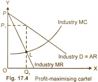
In this figure 17.4,
the industry demand curve DD consisting of three firms is
identical. So is the case with the MR curve and MC curve which
are identical. The cartel's MR curve intersects the MC curve at
point L. Profits are maximized at output OQ1, where
MC = MR. The cartel will set a price OP1, at which OQ1,
output will be demanded.
Having agreed on the
cartel price, the members may then complete each other using non
price competition to gain as big share of resulting sales OQ1
as they can.
There is another
alternative also. The cartel members may agree to divide the
market between them. Each member would given a quota. The sum of
all the quotas must add up to Q1. In case the quotas
exceeded OQ1 either the output will remain unsold at
OP price or the price would fall.
(2)
Price and Output Determination Under Non-Collusive Oligopoly:
It will be explain
with the help of kinked Demand Curve Model.
(i)
The Kinked Demand Curve Model:
The Kinked
demand curve model was developed by Paul Sweezy (1939).
According to him, the firms under oligopoly try to avoid any
activity which could lead to price wars among them. The firms
mostly make efforts to operate in non price competition for
increasing their respective shares of the market and their
profit. An analytical device which is used to explain the
oligopolistic price rigidity is the Kinked Demand Curve.
This model operates
on fulfilling certain conditions which, in brief,
are as under:
(a) All the firms in
the industry are quite developed with or without product
differentiation.
{b} All the firms are
selling the goods on fairly satisfactory price in the market.
(c) If any one firm
lowers the price of its product to capture a larger share of the
market, the other firms follow and reduce the price of their
goods in order to retain their share of the market.
(d) If one firm
raises the price of its goods, the other firms will not follow
the price increase. Some of the customers of the price raising
firm will shift to the relatively low priced firms.
Mr. Paul Sweezy used
two demand curve concepts to explain the model. These are
reproduced below:
Diagram:

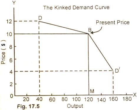
In the figure 17.5.
DD/ is a kinked demand curve. It is made up or two segments DB
and BD/. The demand curve is kinked Or has a bend at point B. The
kink is formed at the prevailing market price level BM ($10
per unit). The segment of the demand curve above the prevailing
price level ($10) is highly elastic and the segment of the
demand curve below the prevailing price level is fairly
inelastic. This is explained now in brief.
Explanation:
Price increase. If an
oligopolistic raises the price of his products from $10 per
unit to $12 per unit, he loses a large part of the market
and his sale comes down to 40 units from 120 units. There is a
loss of 80 units in sale as most of his customers are now
purchasing goods from his competitor firms who are selling the
goods at $10 per units. So an increase in price above the
prevailing level-shows that the demand curve to the left of and
above point B is fairly elastic.
Price reduction. If
an oligopolistic reduces the prices of its goods below the
prevailing price level BM ($10 per unit) for increasing his
sales, his competitors will also match price changes so that
their customers do not go away from them. Let us assume that
Oligopolist has lowered the price to $4.0 per unit. Its
competitors in the industry match the price cut. The sale of the oligopolist with a big price cut of
$.6.0 per unit has
increased by only 40 units (160 - 120 = 40). The firm does not
gain as the total revenue decreases with the price cut. The BD/
portion of the demand curve which lies on the right side and
below point B is fairly inelastic.
Rigid Prices. The
firms in the oligopolist market 'have no incentive to raise or
lower the prices of the goods. They prefer to sell the goods at
the
prevailing price
level due to reaction function. The price BM ($10 per unit)
will, therefore, tend to remain stable or rigid, as every member
of the oligopoly does not see any gain by lowering or raising
the price of his goods.
(3) Price
Leadership
Model:
The firms in the
oligopolistic market are not happy with price competition among
themselves. They try various methods to maximize joint profits.
Price leadership is one of the means which provides relief to
the firms from the strains of price competition.
The firms in the
oligopolistic industry (without any formal agreement) accept the
price set by the leading firm in the industry and move their
prices in line with the prices of the leader firm. The
acceptance of price set by the price leader firm maximizes the
total profits of each firm in the oligopolistic industry.
Assumptions:
The main assumptions
of price leadership model under oligopoly are as under:
(a) There are two
firms A and B in the market.
(b) The output
produced by the two firms is homogeneous.
(c) The firm 'A being
the low cost firm or a dominant firm acts as a leader firm.
(d) Both of the firms
face the same demand curve.
(e) Each of the two
firms has an equal share in the market. The price and output
determination under price leadership is now explained with the
help of the diagram below.
Diagram:

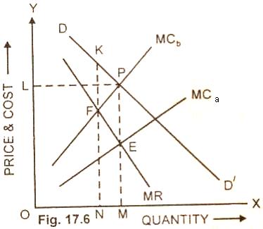
In this figure 1 7.6,
DD/ is the demand curve which is faced by each of the two
firms. MR is the marginal revenue curve of each firm. MCa
is the marginal cost of firm A and MCb is the marginal cost of
firm B. We have assumed that the firm A is a low cost firm than
firm B. As such the MCa lies below MCb.
The leader firm using
the marginalistic rule of MC = MR is in equilibrium at point E.
The firm A maximizes profits by selling output OM and setting
price MP. The firm B
is in equilibrium at point F where MCb = MR.
The firm B
maximizes profits by producing ON output and selling it at NK
price. The firm B has to compete firm A in the market, if the
firm B fixes the price NK per unit, it will not be able to
compete with firm A which is selling goods at MP price per unit.
Hence, the firm B will be compelled to follow the leader firm A.
The firm B will also charge MP price per unit as set by the firm
A. The firm B will also produce QM output like the firm A. Thus
both the firms will charge the same price MP and sell each of
them OM output. The total output will thus be twice of OM.
The firm A being the
low cost firm will maximize profits by selling OM output at MP
price. The profits of the firm B is lower than of firm A because
its costs of production is higher than of firm A.
Conclusion:
After studying the
pricing and output decisions under various forms of oligopoly,
the main conclusion drawn is that allocate and productive
efficiency are unlikely to be achieved under them. However,
Schumpeter's view Is that oligopolists have both the Incentive
and financial and technical resources to be more technological
progressive than competitive firms.