Concept of
Propensity to Save/Saving Function:
Definition:
The
propensity to save schedule which for the sake of brevity is called the
propensity to save or saving function shows relation between saving and
disposable income at varying levels of income S = F(Y).
The propensity to save
schedule comes from subtracting consumption from income at each level of income.
Since saving represents the difference between the 45o guideline and the
consumption function, it may be positive or negative. The propensity to save
schedule can easily be derived from the
propensity
to consume schedule, in our example given earlier, (Click
here to read full example), the propensity to consume, is as follows:
|
Income ($ in billion) |
50 |
100 |
140 |
200 |
300 |
|
Expenditure ($ in billion) |
50 |
70 |
100 |
140 |
200 |
The
propensity to save schedule can easily be derived by subtracting the amount of
consumption from the corresponding amount of income. The saving schedule thus is
as follows:
|
Income ($ in billion) |
50 |
100 |
140 |
200 |
300 |
|
Save ($ in billion) |
0 |
30 |
40 |
60 |
100 |
Concepts of
Propensity to Save:
There are two concepts of
propensity to save:
(1) Average
Propensity to Save (APS).
(2) Marginal
Propensity to
Save (MPS).
(1) Average
Propensity to Save (APS):
Definition:
Average propensity to save is
the percentage of income saved at a given level of income (APS).
The average
propensity to save at any point can be found by dividing saving by income.
For
instance, If the disposable income is $100 billion and expenditure $80
billion on consumption goods, then the saving win be equal to $20 billion. The
average propensity at save will be = 0.2. The average propensity to save can also
be found by subtracting average propensity to consume from 1. In the above
example, the average propensity to consume is:
80/1000 =
0.8
So the average
propensity save will be 1 - 8 = 2
(2)
Marginal Propensity to Save (MPS):
Definition:
Marginal propensity to save is the ratio of change in saving to change
in income. The MPS measures the change in saving generated by a change in
income.
Formula:
MPS =
Change in Saving
Change in Income
MPS = ΔS
ΔY
It is also found out by
subtracting marginal propensity to
consume from 1. Thus:
MPS = 1 - MPC
Schedule
For APS and MPS:
($ in billion)
|
Disposable Income
(Y) |
Consumption Expenditure (C) |
Net Saving (S) |
Average Propensity to Save
(1 (1 - PC = PS) |
Marginal Propensity to Save
(1 - MPC = MPS) |
| A
1000 |
1100 |
$100 |
1
-1 = 1 |
1
- 9 = 0.1 |
| B
2000 |
2000 |
$000 |
1
- 1 = 0 |
1
- 6 = 0.4 |
| C
3000 |
2600 |
$400 |
1
- 0.86 = 0.14 |
1
- 5 = 0.5 |
| D
4000 |
3100 |
$900 |
1
- 0.77 = 0.23 |
1
- 3 = 0.7 |
| E
5000 |
3400 |
$1600 |
1
- 0.68 = 0.32 |
1
- 2 = 0.8 |
| F
6000 |
3600 |
$2400 |
1
- 0.6 = 0.4 |
1
- 1 = 0.9 |
| G
7000 |
3700 |
$3300 |
1
- 0.53 = 0.47 |
|
It is quite clear from the above saving schedule that as
the income increases, the average propensity to save and marginal propensity to
save also increases and as income decreases, the average propensity to save and
the marginal propensity to save also decreases.
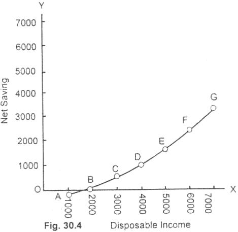
Diagram:

In figure (30.4) disposable income is measured along the X
axis and saving along the Y axis. At point A, the consumption expenditure
$1,100 billion against the disposable income of $1,000 billion. The
expenditure is more than the disposable income. There is dis-saving of $100 billion. The excess expenditure of
$100 billion is met either out of
accumulated saving or by borrowing. When income increases to $2,000 billion,
the expenditure also increases to $2,000 billion.
At point B, consumption is
exactly equal to expenditure. B is the break even point where C =Y. From B onward up to G point, saving goes or increasing with the increase in disposable income.
AG thus is the saving curve which has risen with the rise in income.
It may
here be noted saving as used by Keynes in consumption function is "real
saving" and ‘income is "real disposable income". The
saving function like the consumption function remain stable in the short period.
Relevant Articles:
|