Home » Determinants of the Level of National Income and Employment » Propensity to Consume

Propensity to Consume:

Meaning and Definition of Propensity to Consume:

The classical economists were of the view that the supply of saving was determined by the rate of interest prevailing in the country. According to them, the higher the rate of interest, the larger is the saving and so less is the consumption.

Keynes disagreed with the above view. According to him interest is not the primary determinant of an individual’s saving and consumption decisions. It is primarily the individual’s real income which determines his, saving and consumption decisions. J.M. Keynes has developed two concepts:

(i) Average Propensity to Consume.

(ii) Marginal Propensity to Consume to Analyze the Consumption Function.

Explanation:

These two concepts are now explained in brief:

(1) Average Propensity to Consume (APC):

Average propensity to consume ( APC) may be defined as:

Definition:

"A ratio of total consumption to total disposable income for different levels of disposable income It is calculated by dividing the amount of consumption by disposable income for any given level of income".

Example:

For instance, when nation’s disposable income is $2,000 billion, consumption expenditure is $1,500 billion, the average propensity to consumption is 1500/2000 = 0.75.

This shows that out of the disposable income of $2,000 billion, 75% will be used for consumption purposes. The APC declines as income increases because the proportion of income spent on consumption decreases. The average propensity to consume spent on consumption decreases. The average propensity to consume at any level of income is expressed in equation as C/Y. Here C stands for consumption Y for income.

Formula:

APC = C

           Y

Diagram:

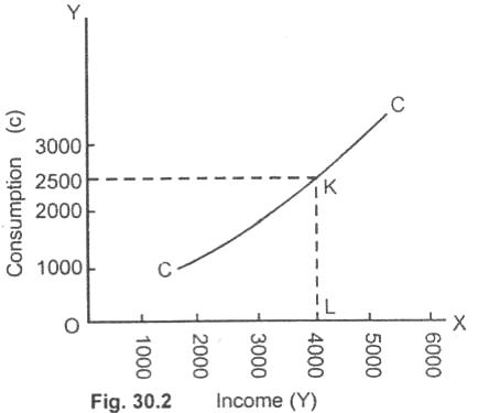
In the Fig.(30.2) income is plotted on OX axis and consumption along OY. CC curve represents the propensity to consume schedule. At point K, the average propensity to consume is equal to 0.62.

KL/OL = (C/Y) i.e., 2500/4000 or 25/40 = 0.62

APC implies a point on the curve C which indicates the ratio of income consumed. The C curve is made up of a series such points.

(2) Marginal Propensity to Consume (MPC):

Definition:

The concept of marginal propensity to consume is very important is macro economics. J.M. Keynes has defined marginal propensity to consume (MPC):

"As the relationship between a change in consumption (ΔC) that resulted from a change in disposable income (ΔY)".

Formula:

It is found out by dividing change in consumption to a given change in disposable Income.

MPC = Change in Consumption = ΔC

                                                                    Change in Income         ΔY

Example:

Thus we make this concept clear by taking an example, let us suppose the disposable income rises from $2000 billion to $3000 billion ( by $1000 billion) and the consumption expenditure increases from $1500 billion to $2000 billion (by $500 billion). The marginal propensity to consume is:

ΔC/ΔY = 500/1000 = 1/2 = 0.5

All the concepts of consumption function are now explained whit help of schedule and a diagram.

Schedule For Propensity to Consume:

($ in billion)

The reader can easily understand from the above schedule that with the increase in the disposable income, the propensity to consume decreases and conversely with a fall in income, the propensity to consume and the marginal propensity to consume increases. The consumption schedule can also be explained with the help of a curve which is given below:

Diagram For Propensity to Consume:

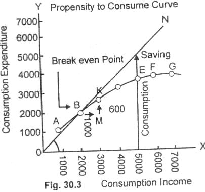
In the figure (30.3), disposable income is measured along the horizontal axis OX and consumption along the vertical axis OY. Let us now draw 45⁰ helping line from O to ON. If we take any point on the 45⁰ helping line, income will be exactly equal to expenditure. The curve AG represents the income consumption schedule, indicating the propensity to consumer at various levels of income. Point A which is above 45⁰ helping line, shows us that the expenditure is greater than its income.

This deficit in income can be converted either by borrowing or from the sale of assets. At point B, consumption expenditures exactly equal to disposable income and there is neither saving nor dis-saving. This point is known is as break even point.

From B onward up to G, the curve lies below the 45⁰ helping line. This shows that the consumption expenditure is less than the disposable income. Net saving is measured by the distance from the propensity to consume curve up to 45⁰ helping line.

For example, when the income is $5,000 billion, the expenditure is $3400 billion and saving $1,600 billion.

Marginal propensity to consume curve can also be illustrated from the very same figure. At point B, income is $2,000 billion and is equal to expenditure, i.e., $2,000. When income increases from $2,000 billion to $3,000 billion, consumption increases only by $600 billion.

Now we move from point B towards right up by $1,000 billion. BM line shows as the increases in income. Then we go vertically until we reach point K. MK line indicates addition made to the total consumption. It is equal to $600 billion. So the marginal propensity to consume will be equal to $600/$1000 = $6.

Relevant Articles:

A D V E R T I S E M E N T

A D V E R T I S E M E N T

All the material on this site is the property of economicsconcepts.com. No part of this website may be reproduced without permission of economics concepts.
All rights reserved Copyright © 2010 - 2015