Short Run
Equilibrium of the Price Taker Firm Under Perfect Competition:
Definition and Explanation:
By short run is meant a
length of time which is not enough to change the level of fixed
inputs or the number of firms in the industry but long enough to
change the level of output by changing variable inputs.
In short
period, a distinction is made of two types of costs (i) fixed
cost and (ii) variable cost.
The fixed cost in the form of fixed
factors i.e., plant, machinery, building, etc. does not vary
with the change in the output of the firm. If the firm is to
increase or decrease its output, the change only takes place in
the quantity of variable resources such as labor, raw material,
etc.
Further, in the short run, the demand curve
facing the firm is horizontal. No new firms enter or leave the
industry. The number of firms in the industry, therefore, remain
the same. Under
perfect
competition, the firm takes the price of the product as
determined in the market. The firm sells all its output at the
prevailing market price. The firm, in other words, is a
price taker.
Equilibrium
of a Competitive Firm:
The short-run equilibrium of a firm
can be easily explained with the help of marginal revenue = marginal cost approach or
(MR = MC)
rule.
Marginal revenue is the change in total revenue that
occurs in response to a one unit change in the quantity sold.
Marginal cost is the addition to total cost resulting from the
additional of marginal unit. Since price is given for the
competitive firm, the average revenue curve of a price taker
firm is identical to the marginal curve. Average revenue (AR)
thus is equal to marginal revenue (MR) is equal to price (MR =
AR = Price).
According to the marginal revenue
and marginal cost approach or (MR = MC) rule , a price taker
firm is in equilibrium at a point where marginal revenue (MR) or
price is equal to marginal cost The point where MR = MC = Price,
the firm produces the best level of output. From this it may not
be concluded that the perfectly competitive firm at the
equilibrium level of output (MR = MC = Price) necessarily
ensures maximum profit. The fact is that in the short period, a
firm at the equilibrium level of output is faced with four types
of product prices in the market which give rise to following
results:
(i) A firm earns supernormal
profits.
(ii) A firm earns normal profits.
(iii) A firm incurs losses but does
not close down.
(iv) A firm minimizes losses by
shutting down. All these short run cases of profits or losses
are explained with the help of diagrams.
Determining
Profit from a Graph:
(1) Profit Maximizing Position:
A firm in the short run earns
abnormal profits when at the best level of output, the market
price exceeds the short run average total cost (SATC). The short
run profit maximizing position of a purely competitive firm is
explained with the help of a diagram.
Diagram/Graph:

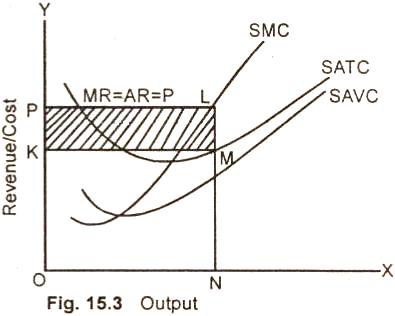
In the figure (15.3), output is
measured along OX axis and revenue / cost on OY axis. We assume
here that the market price is equal to OP. A price taker firm
has to sell its entire output at this prevailing market price
i.e. OP. The firm is in equilibrium at point L. Where MC = MR.
The inter section of MC and MR determine the quantity of the
good the firm will produce.
After having determined the
quantity, drop a vertical line down to the horizontal axis and
see what the average total cost (ATC) is at that output level
(point N). The competitive firm will produce ON quantity of
output and sell at market price OP. The total revenue of the
firm at the best level of output ON is equal to OPLN. Whereas
the total cost of producing ON quantity of output is equal to
OKMN. The firm is earning supernormal profits equal to the
shaded rectangle KPLM. The per unit profit is indicated by the
distance LM or PK.
It may here be noted that a firm
would not produce more than ON units because producing another
unit adds more to the cost than the firm would receive from the
sale of the unit (MC > MR). The firm would not stop short of ON
output because producing another unit adds more to the revenue
than to cost (MR > MC). Hence, ON is the best level of
output where profit of the firm is maximum.
(2) Zero
Profit of a Firm:
A firm, in the short run, may be
making zero economic profit or normal economic profit. It may
here be remembered that although economic profit is zero, all
the resources including entrepreneurs are being paid their
opportunity. So they are getting a normal profit the
case of normal profits of a firms at break even price is
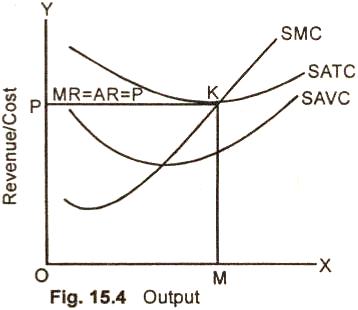
explained with the help of the diagram 15.4.

We assume in the figure (15.4) that
OP is the prevailing market price and PK is the average revenue,
marginal revenue curve. At point K, which is the break even
price for a Competitive firm, the MR, MC and ATC are all equal.
The firm produces OM output-and sells at market price OP. The
total revenue of the firm to equal is the area OPKM. The total
cost of producing OM output also equals the area OPKM. The firm
is earning only normal profits. It is a situation in which the
resources employed by the firm are earning just what they
could-earn in some other alternative occupations.
(3) Loss
Minimizing Case:
The firm in the short rue is
minimizing tosses if the market price is smaller than average
total cost but larger than average variable cost. The loss
minimizing position of a price taker firm is explained with the
help of a diagram.

We assume in the figure (15.5) that
the market price is QP. The firm is in equilibrium at point N
where MR = MC. The firm's best level of output is OK which is
sold at unit cost OP. The total revenue of the firm is equal to
the area OPNK. The total cost of producing OK quantity of output
is equal to OTSK. The firm is suffering a net loss equal to the
shaded area PTSN.
The firm at price OP in the market
is covering its full variable cost and a part of the fixed cost.
The loss of part of fixed cost equal to the shaded area PTSN is
less than, the firm would incur by closing down. In case of shut
down, the firm has to bear the total fixed cost ETSF. The firm
thus by producing OK output and selling at OP price is
minimizing losses. Summing up, in the short run the firm will
not go out of business for as long as the loss m staying the
business is less than the loss from closing down.
(4) Short Run Shut Down:
The price taker firm in the
short-run minimizes losses by closing it down if the market
price is less than average variable cost. The shut down position
of a Competitive firm is explained with the help of a diagram.

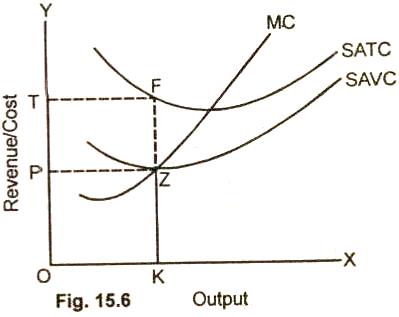
In this figure (15.6) we assume that
the market price is OP. The firm, is in equilibrium at point Z
where MR = MC. The firm produces OK output and sells at OP unit
cost. The total revenue of the firm is equal to the area OPZK.
Whereas .the total cost producing OK output is OTFR. The firm is
suffering a net loss of total fixed cost equal to the area PTFZ.
The firm at point Z is just covering average variable costs.
If the price falls below Z, the
competitive firm will minimize its losses by closing down. There
is no level of output which the firm can produce and realize a
loss smaller than its fixed costs. It is therefore a shut
down point for the firm. Operate When Price is > average
variable cost.
Relevant Articles:
|